5 Getting acquainted with R

In this chapter we will use R to read a dataset and produce some descriptive statistics, produce some charts, and perform some simple statistical inference. The aim of the exercise is for you to become familiar with R and some basic R functions and objects.

The first thing we will do, after starting R, is issue a command to retrieve an example dataset:

fem <- read.table("fem.dat", header = TRUE)

This command illustrates some key things about the way R works.

We are instructing R to assign (using the <- operator) the output of the read.table() function to an object called fem.

The fem object will contain the data held in the file fem.dat as an R data.frame object:

class(fem)

[1] "data.frame"

You can inspect the contents of the fem data.frame (or any other R object) just by typing its name:

fem

  ID AGE IQ ANX DEP SLP SEX LIFE    WT
1  1  39 94   2   2   2   1    1  2.23
2  2  41 89   2   2   2   1    1  1.00
3  3  42 83   3   3   2   1    1  1.82
4  4  30 99   2   2   2   1    1 -1.18
5  5  35 94   2   1   1   1    2 -0.14
6  6  44 90  NA   1   2   2    2  0.41

Note that the fem object is built from other objects. These are the named vectors (columns) in the dataset:

names(fem)

[1] "ID"   "AGE"  "IQ"   "ANX"  "DEP"  "SLP"  "SEX"  "LIFE" "WT"

The [1] displayed before the column names refers to the numbered position of the first name in the output. These positions are known as indexes and can be used to refer to individual items. For example:

names(fem)[1]

[1] "ID"

names(fem)[8]

[1] "LIFE"

names(fem)[2:4]

[1] "AGE" "IQ"  "ANX"

The data consist of 118 records:

nrow(fem)

[1] 118

each with nine variables:

ncol(fem)

[1] 9

for female psychiatric patients.

The columns in the dataset are:

ID	Patient ID
AGE	Age in years
IQ	IQ score
ANX	Anxiety (1=none, 2=mild, 3=moderate, 4=severe)
DEP	Depression (1=none, 2=mild, 3=moderate or severe)
SLP	Sleeping normally (1=yes, 2=no)
SEX	Lost interest in sex (1=yes, 2=no)
LIFE	Considered suicide (1=yes, 2=no)
WT	Weight change (kg) in previous 6 months

The first ten records of the fem data.frame are:

   ID AGE  IQ ANX DEP SLP SEX LIFE    WT
1   1  39  94   2   2   2   1    1  2.23
2   2  41  89   2   2   2   1    1  1.00
3   3  42  83   3   3   2   1    1  1.82
4   4  30  99   2   2   2   1    1 -1.18
5   5  35  94   2   1   1   1    2 -0.14
6   6  44  90  NA   1   2   2    2  0.41
7   7  31  94   2   2  NA   1    1 -0.68
8   8  39  87   3   2   2   1    2  1.59
9   9  35 -99   3   2   2   1    1 -0.55
10 10  33  92   2   2   2   1    1  0.36

You may check this by asking R to display all columns of the first ten records in the fem data.frame:

fem[1:10, ]

   ID AGE  IQ ANX DEP SLP SEX LIFE    WT
1   1  39  94   2   2   2   1    1  2.23
2   2  41  89   2   2   2   1    1  1.00
3   3  42  83   3   3   2   1    1  1.82
4   4  30  99   2   2   2   1    1 -1.18
5   5  35  94   2   1   1   1    2 -0.14
6   6  44  90  NA   1   2   2    2  0.41
7   7  31  94   2   2  NA   1    1 -0.68
8   8  39  87   3   2   2   1    2  1.59
9   9  35 -99   3   2   2   1    1 -0.55
10 10  33  92   2   2   2   1    1  0.36

The space after the comma is optional. You can think of it as a placeholder for where you would specify the indexes for columns you wanted to display. For example:

fem[1:10,2:4]

displays the first ten rows and the second, third and fourth columns of the fem data.frame:

   AGE  IQ ANX
1   39  94   2
2   41  89   2
3   42  83   3
4   30  99   2
5   35  94   2
6   44  90  NA
7   31  94   2
8   39  87   3
9   35 -99   3
10  33  92   2

NA is a special value meaning not available or missing.

You can access the contents of a single column by name:

fem$IQ

  [1]  94  89  83  99  94  90  94  87 -99  92  92  94  91  86  90 -99  91  82
 [19]  86  88  97  96  95  87 103 -99  91  87  91  89  92  84  94  92  96  96
 [37]  86  92 102  82  92  90  92  88  98  93  90  91 -99  92  92  91  91  86
 [55]  95  91  96 100  99  89  89  98  98 103  91  91  94  91  85  92  96  90
 [73]  87  95  95  87  95  88  94 -99 -99  87  92  86  93  92 106  93  95  95
 [91]  92  98  92  88  85  92  84  92  91  86  92  89 -99  96  97  92  92  98
[109]  91  91  89  94  90  96  87  86  89 -99

fem$IQ[1:10]

 [1]  94  89  83  99  94  90  94  87 -99  92

The $ sign is used to separate the name of the data.frame and the name of the column of interest. Note that R is case-sensitive so that IQ and iq are not the same.

You can also access rows, columns, and individual cells by specifying row and column positions. For example, the IQ column is the third column in the fem data.frame:

fem[ ,3]

  [1]  94  89  83  99  94  90  94  87 -99  92  92  94  91  86  90 -99  91  82
 [19]  86  88  97  96  95  87 103 -99  91  87  91  89  92  84  94  92  96  96
 [37]  86  92 102  82  92  90  92  88  98  93  90  91 -99  92  92  91  91  86
 [55]  95  91  96 100  99  89  89  98  98 103  91  91  94  91  85  92  96  90
 [73]  87  95  95  87  95  88  94 -99 -99  87  92  86  93  92 106  93  95  95
 [91]  92  98  92  88  85  92  84  92  91  86  92  89 -99  96  97  92  92  98
[109]  91  91  89  94  90  96  87  86  89 -99

fem[9, ]

  ID AGE  IQ ANX DEP SLP SEX LIFE    WT
9  9  35 -99   3   2   2   1    1 -0.55

fem[9,3]

[1] -99

There are missing values in the IQ column which are all coded as -99. Before proceeding we must set these to the special NA value:

fem$IQ[fem$IQ == -99] <- NA

The term inside the square brackets is also an index. This type of index is used to refer to subsets of data held in an object that meet a particular condition. In this case we are instructing R to set the contents of the IQ variable to NA if the contents of the IQ variable is -99.

Check that this has worked:

fem$IQ

  [1]  94  89  83  99  94  90  94  87  NA  92  92  94  91  86  90  NA  91  82
 [19]  86  88  97  96  95  87 103  NA  91  87  91  89  92  84  94  92  96  96
 [37]  86  92 102  82  92  90  92  88  98  93  90  91  NA  92  92  91  91  86
 [55]  95  91  96 100  99  89  89  98  98 103  91  91  94  91  85  92  96  90
 [73]  87  95  95  87  95  88  94  NA  NA  87  92  86  93  92 106  93  95  95
 [91]  92  98  92  88  85  92  84  92  91  86  92  89  NA  96  97  92  92  98
[109]  91  91  89  94  90  96  87  86  89  NA

We can now compare the groups who have and have not considered suicide. For example:

by(fem$IQ, fem$LIFE, summary)

Look at the help for the by() function:

help(by)

Note that you may use ?by as a shortcut for help(by).

The by() function applies another function (in this case the summary() function) to a column in a data.frame (in this case fem$IQ) split by the value of another variable (in this case fem$LIFE).

It can be tedious to always have to specify a data.frame each time we want to use a particular variable. We can fix this problem by ‘attaching’ the data.frame:

attach(fem)

We can now refer to the columns in the fem data.frame without having to specify the name of the data.frame. This time we will produce summary statistics for WT by LIFE:

by(WT, LIFE, summary)

LIFE: 1
   Min. 1st Qu.  Median    Mean 3rd Qu.    Max.    NA's 
-2.2300 -0.2700  1.0000  0.7867  1.7300  3.7700       4 
------------------------------------------------------------ 
LIFE: 2
   Min. 1st Qu.  Median    Mean 3rd Qu.    Max.    NA's 
-1.6800 -0.4500  0.6400  0.6404  1.5000  2.9500       7

We can view the same data as a box and whisker plot:

boxplot(WT ~ LIFE)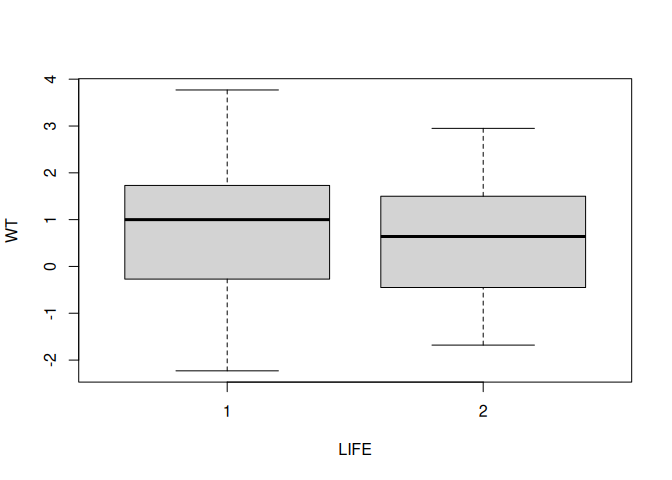

We can add axis labels and a title to the graph:

boxplot(
  WT ~ LIFE,
  xlab = "Life",
  ylab = "Weight",
  main = "Weight BY Life"
)

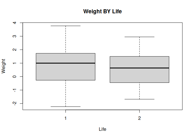
A more descriptive title might be “Weight Change BY Considered Suicide”.

The groups do not seem to differ much in their medians and the distributions appear to be reasonably symmetrical about their medians with a similar spread of values.

We can look at the distribution as histograms:

hist(WT[LIFE == 1])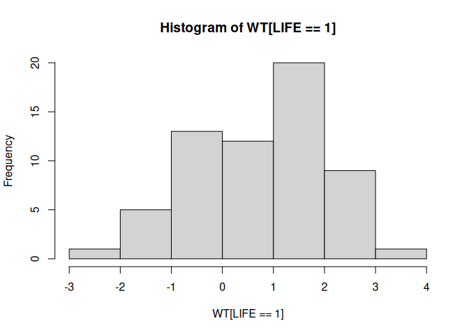

hist(WT[LIFE == 2])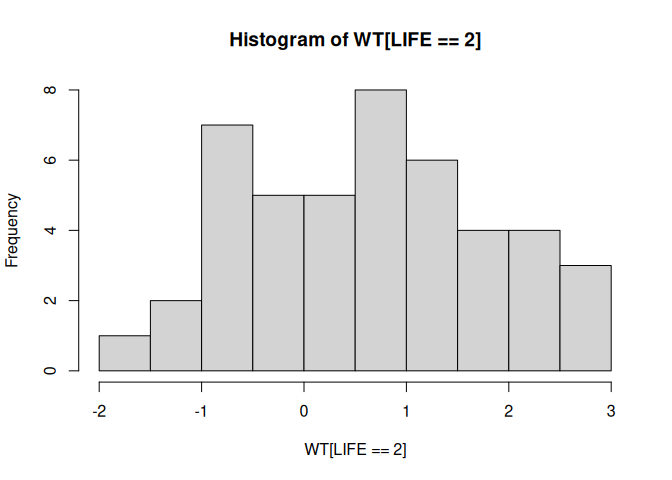

and check the assumption of normality using quantile-quantile plots:

qqnorm(WT[LIFE == 1])
qqline(WT[LIFE == 1])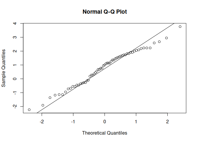

qqnorm(WT[LIFE == 2])
qqline(WT[LIFE == 2])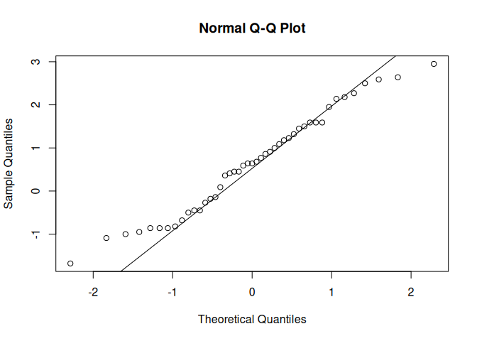

or by using a formal test:

shapiro.test(WT[LIFE == 1])


    Shapiro-Wilk normality test

data:  WT[LIFE == 1]
W = 0.98038, p-value = 0.4336

shapiro.test(WT[LIFE == 2])


    Shapiro-Wilk normality test

data:  WT[LIFE == 2]
W = 0.97155, p-value = 0.3292

Remember that we can use the by() function to apply a function to a data.frame, including statistical functions such as shapiro.test():

by(WT, LIFE, shapiro.test)

LIFE: 1

    Shapiro-Wilk normality test

data:  dd[x, ]
W = 0.98038, p-value = 0.4336

------------------------------------------------------------ 
LIFE: 2

    Shapiro-Wilk normality test

data:  dd[x, ]
W = 0.97155, p-value = 0.3292

We can also test whether the variances differ significantly using Bartlett’s test for the homogeneity of variances:

bartlett.test(WT, LIFE)


    Bartlett test of homogeneity of variances

data:  WT and LIFE
Bartlett's K-squared = 0.32408, df = 1, p-value = 0.5692

There is no significant difference between the two variances.

Many functions in R have a formula interface that may be used to specify multiple variables and the relations between multiple variables. We could have used the formula interface with the bartlett.test() function:

bartlett.test(WT ~ LIFE)


    Bartlett test of homogeneity of variances

data:  WT by LIFE
Bartlett's K-squared = 0.32408, df = 1, p-value = 0.5692

Having checked the normality and homogeneity of variance assumptions we can proceed to carry out a t-test:

t.test(WT ~ LIFE, var.equal = TRUE)


    Two Sample t-test

data:  WT by LIFE
t = 0.59869, df = 104, p-value = 0.5507
alternative hypothesis: true difference in means between group 1 and group 2 is not equal to 0
95 percent confidence interval:
 -0.3382365  0.6307902
sample estimates:
mean in group 1 mean in group 2 
      0.7867213       0.6404444

There is no evidence that the two groups differ in weight change in the previous six months.

We could still have performed a t-test if the variances were not homogenous by setting the var.equal parameter of the t.test() function to FALSE:

t.test(WT ~ LIFE, var.equal = FALSE)


    Welch Two Sample t-test

data:  WT by LIFE
t = 0.60608, df = 98.866, p-value = 0.5459
alternative hypothesis: true difference in means between group 1 and group 2 is not equal to 0
95 percent confidence interval:
 -0.3326225  0.6251763
sample estimates:
mean in group 1 mean in group 2 
      0.7867213       0.6404444

or performed a non-parametric test:

wilcox.test(WT ~ LIFE)


    Wilcoxon rank sum test with continuity correction

data:  WT by LIFE
W = 1488, p-value = 0.4622
alternative hypothesis: true location shift is not equal to 0

An alternative, and more general, non-parametric test is:

kruskal.test(WT ~ LIFE)


    Kruskal-Wallis rank sum test

data:  WT by LIFE
Kruskal-Wallis chi-squared = 0.54521, df = 1, p-value = 0.4603

We can use the table() function to examine the differences in depression between the two groups:

table(DEP, LIFE)

The two distributions look very different from each other. We can test this using a chi-square test on the table:

chisq.test(table(DEP, LIFE))


    Pearson's Chi-squared test

data:  table(DEP, LIFE)
X-squared = 43.876, df = 2, p-value = 2.968e-10

Note that we passed the output of the table() function directly to the chisq.test() function. We could have saved the table as an object first and then passed the object to the chisq.test() function:

tab <- table(DEP, LIFE)
chisq.test(tab)


    Pearson's Chi-squared test

data:  tab
X-squared = 43.876, df = 2, p-value = 2.968e-10

The tab object contains the output of the table() function:

class(tab)

[1] "table"

tab

We can pass this table object to another function. For example:

fisher.test(tab)


    Fisher's Exact Test for Count Data

data:  tab
p-value = 1.316e-12
alternative hypothesis: two.sided

When we are finished with the tab object we can delete it using the rm() function:

rm(tab)

You can see a list of available objects using the ls() function:

ls()

[1] "fem"             "pandoc_dir"      "quarto_bin_path"

This should just show the fem object.

We can examine the association between loss of interest in sex and considering suicide in the same way:

tab <- table(SEX, LIFE)
tab

fisher.test(tab)


    Fisher's Exact Test for Count Data

data:  tab
p-value = 0.03175
alternative hypothesis: true odds ratio is not equal to 1
95 percent confidence interval:
  1.080298 14.214482
sample estimates:
odds ratio 
  3.620646

Note that with a two-by-two table the fisher.test() function produces an estimate of, and confidence intervals for, the odds ratio. Again, we will delete the tab object:

rm(tab)

We could have performed the Fisher exact test without creating the tab object by passing the output of the table() function directly to the fisher.test() function:

fisher.test(table(SEX, LIFE))


    Fisher's Exact Test for Count Data

data:  table(SEX, LIFE)
p-value = 0.03175
alternative hypothesis: true odds ratio is not equal to 1
95 percent confidence interval:
  1.080298 14.214482
sample estimates:
odds ratio 
  3.620646

Choose whichever method you find easiest but remember that it is easy to save the results of any function for later use.

We can explore the correlation between two variables using the cor() function:

cor(IQ, WT, use = "pairwise.complete.obs")

[1] -0.2917158

or by using a scatter plot:

plot(IQ, WT)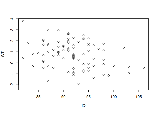

and by a formal test:

cor.test(IQ, WT)


    Pearson's product-moment correlation

data:  IQ and WT
t = -3.0192, df = 98, p-value = 0.003231
alternative hypothesis: true correlation is not equal to 0
95 percent confidence interval:
 -0.4616804 -0.1010899
sample estimates:
       cor 
-0.2917158

With some functions you can pass an entire data.frame rather than a list of variables:

cor(fem, use = "pairwise.complete.obs")
pairs(fem)

              ID         AGE            IQ         ANX           DEP
ID    1.00000000  0.03069077  0.0370598672 -0.02941825 -0.0554147209
AGE   0.03069077  1.00000000 -0.4345435680  0.06734300 -0.0387049246
IQ    0.03705987 -0.43454357  1.0000000000 -0.02323787 -0.0001307404
ANX  -0.02941825  0.06734300 -0.0232378691  1.00000000  0.5437946347
DEP  -0.05541472 -0.03870492 -0.0001307404  0.54379463  1.0000000000
SLP  -0.07268743  0.02606547  0.0812993104  0.22317875  0.5248724551
SEX   0.08999634  0.10609216 -0.0536558660 -0.21062493 -0.3058422258
LIFE -0.05604349 -0.10300193 -0.0915396469 -0.34211268 -0.6139017253
WT    0.02640131  0.41574411 -0.2917157832  0.11817532  0.0233742465
              SLP         SEX        LIFE           WT
ID   -0.072687434  0.08999634 -0.05604349  0.026401310
AGE   0.026065468  0.10609216 -0.10300193  0.415744109
IQ    0.081299310 -0.05365587 -0.09153965 -0.291715783
ANX   0.223178752 -0.21062493 -0.34211268  0.118175321
DEP   0.524872455 -0.30584223 -0.61390173  0.023374247
SLP   1.000000000 -0.29053971 -0.35186578 -0.009259774
SEX  -0.290539709  1.00000000  0.22316967 -0.027826514
LIFE -0.351865775  0.22316967  1.00000000 -0.058605326
WT   -0.009259774 -0.02782651 -0.05860533  1.000000000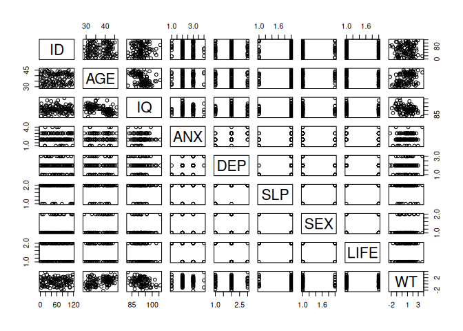

The output can be a little confusing particularly if it includes categorical or record identifying variables. To avoid this we can create a new object that contains only the columns we are interested in using the column binding cbind() function:

newfem <- cbind(AGE, IQ, WT)
cor(newfem, use = "pairwise.complete.obs")
pairs(newfem)

           AGE         IQ         WT
AGE  1.0000000 -0.4345436  0.4157441
IQ  -0.4345436  1.0000000 -0.2917158
WT   0.4157441 -0.2917158  1.0000000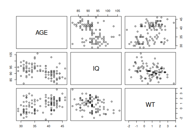

When we have finished with the newfem object we can delete it:

rm(newfem)

There was no real need to create the newfem object as we could have fed the output of the cbind() function directly to the cor() or pairs() function:

cor(cbind(AGE, IQ, WT), use = "pairwise.complete.obs")
pairs(cbind(AGE, IQ, WT))

           AGE         IQ         WT
AGE  1.0000000 -0.4345436  0.4157441
IQ  -0.4345436  1.0000000 -0.2917158
WT   0.4157441 -0.2917158  1.0000000

It is, however, easier to work with the newfem object rather than having to retype the cbind() function. This is particularly true if you wanted to continue with an analysis of just the three variables.

The relationship between AGE and WT can be plotted using the plot() function:

plot(AGE, WT)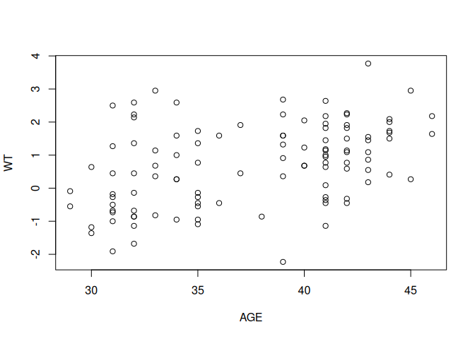

And tested using the cor() and cor.test() functions:

cor(AGE, WT, use = "pairwise.complete.obs")

[1] 0.4157441

cor.test(AGE, WT)


    Pearson's product-moment correlation

data:  AGE and WT
t = 4.6841, df = 105, p-value = 8.457e-06
alternative hypothesis: true correlation is not equal to 0
95 percent confidence interval:
 0.2452434 0.5612979
sample estimates:
      cor 
0.4157441

Or by using the linear modelling lm() function:

summary(lm(WT ~ AGE))


Call:
lm(formula = WT ~ AGE)

Residuals:
     Min       1Q   Median       3Q      Max 
-3.10678 -0.85922 -0.05453  0.71434  2.70874 

Coefficients:
            Estimate Std. Error t value Pr(>|t|)    
(Intercept) -3.25405    0.85547  -3.804  0.00024 ***
AGE          0.10592    0.02261   4.684 8.46e-06 ***
---
Signif. codes:  0 '***' 0.001 '**' 0.01 '*' 0.05 '.' 0.1 ' ' 1

Residual standard error: 1.128 on 105 degrees of freedom
  (11 observations deleted due to missingness)
Multiple R-squared:  0.1728,    Adjusted R-squared:  0.165 
F-statistic: 21.94 on 1 and 105 DF,  p-value: 8.457e-06

We use the summary() function here to extract summary information from the output of the lm() function.

It is often more useful to use lm() to create an object:

fem.lm <- lm(WT ~ AGE)

And use the output in other functions:

summary(fem.lm)


Call:
lm(formula = WT ~ AGE)

Residuals:
     Min       1Q   Median       3Q      Max 
-3.10678 -0.85922 -0.05453  0.71434  2.70874 

Coefficients:
            Estimate Std. Error t value Pr(>|t|)    
(Intercept) -3.25405    0.85547  -3.804  0.00024 ***
AGE          0.10592    0.02261   4.684 8.46e-06 ***
---
Signif. codes:  0 '***' 0.001 '**' 0.01 '*' 0.05 '.' 0.1 ' ' 1

Residual standard error: 1.128 on 105 degrees of freedom
  (11 observations deleted due to missingness)
Multiple R-squared:  0.1728,    Adjusted R-squared:  0.165 
F-statistic: 21.94 on 1 and 105 DF,  p-value: 8.457e-06

plot(AGE, WT)
abline(fem.lm)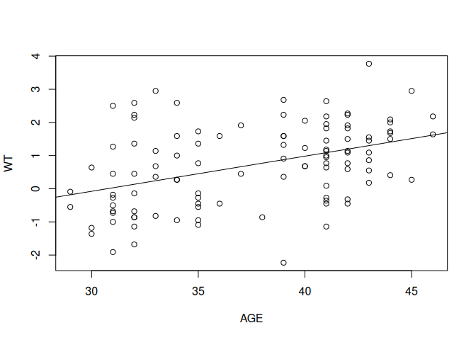

In this case we are passing the intercept and slope information held in the fem.lm object to the abline() function which draws a regression line. The abline() function adds to an existing plot. This means that you need to keep the scatter plot of AGE and WT open before issuing the abline() function call.

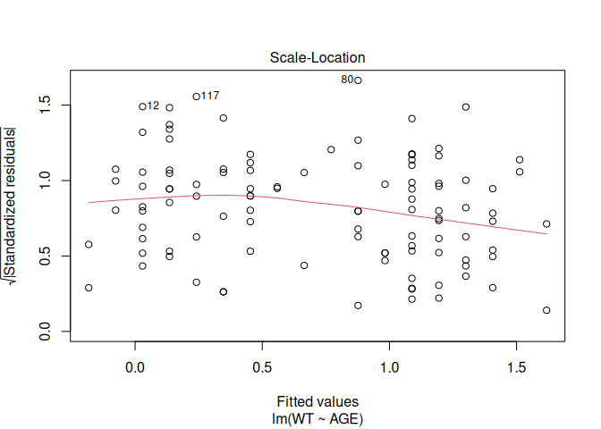
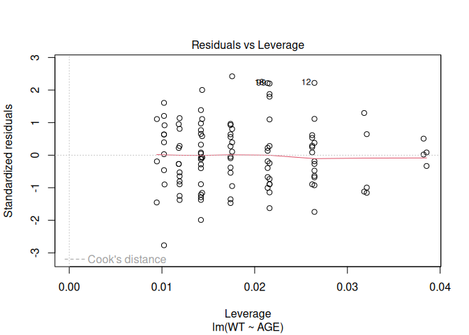
A useful function to apply to the fem.lm object is plot() which produces diagnostic plots of the linear model:

plot(fem.lm)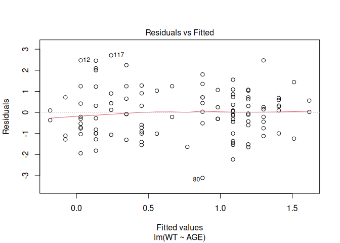

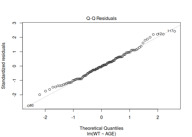
Objects created by the lm() function (or any of the modelling functions) can use up a lot of memory so we should remove them when we no longer need them:

rm(fem.lm)

It might be interesting to see whether a similar relationship exists between AGE and WT for those who have and have not considered suicide. This can be done using the coplot() function:

coplot(WT ~ AGE | as.factor(LIFE))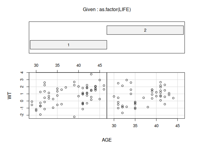


 Missing rows: 21, 22, 31, 43, 44, 45, 69, 81, 101, 104, 114, 115

The two plots looks similar. We could also use coplot() to investigate the relationship between AGE and WT for categories of both LIFE and SEX:

coplot(WT ~ AGE | as.factor(LIFE) * as.factor(SEX))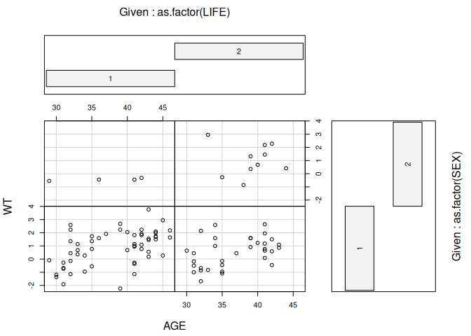


 Missing rows: 12, 17, 21, 22, 31, 43, 44, 45, 66, 69, 81, 101, 104, 105, 114, 115

although the numbers are too small for this to be useful here.

We used the as.factor() function with the coplot() function to ensure that R was aware that the LIFE and SEX columns hold categorical data.

We can check the way variables are stored using the data.class() function:

data.class(fem$SEX)

[1] "numeric"

The parameters of most R functions have default values. These are usually the most used and most useful parameter values for each function. The cor.test() function, for example, calculates Pearson’s product moment correlation coefficient by default. This is an appropriate measure for data from a bivariate normal distribution. The DEP and ANX variables contain ordered data. An appropriate measure of correlation between DEP and ANX is Kendall’s tau. This can be obtained using:

cor.test(DEP, ANX, method = "kendall")


    Kendall's rank correlation tau

data:  DEP and ANX
z = 5.5606, p-value = 2.689e-08
alternative hypothesis: true tau is not equal to 0
sample estimates:
      tau 
0.4950723

5.1 Summary

R is a functional system. Everything is done by calling functions.
R provides a large set of functions for descriptive statistics, charting, and statistical inference.
Functions can be chained together so that the output of one function is the input of another function.
R is an object oriented system. We can use functions to create objects that can then be manipulated or passed to other functions for subsequent analysis.